
Get 50% off the “Data Science at the Command Line” ebook with code DATA50.
Editor’s Note: This post is a slightly adapted excerpt from Jeroen Janssens’ recent book, “Data Science at the Command Line.” To follow along with the code, and learn more about the various tools, you can install the Data Science Toolbox, a free virtual machine that runs on Microsoft Windows, Mac OS X, and Linux, and has all the command-line tools pre-installed.
The goal of dimensionality reduction is to map high-dimensional data points onto a lower dimensional space. The challenge is to keep similar data points close together on the lower-dimensional mapping. As we’ll see in the next section, our data set contains 13 features. We’ll stick with two dimensions because that’s straightforward to visualize.
Dimensionality reduction is often regarded as being part of the exploring step. It’s useful for when there are too many features for plotting. You could do a scatter plot matrix, but that only shows you two features at a time. It’s also useful as a preprocessing step for other machine-learning algorithms. Most dimensionality reduction algorithms are unsupervised, which means that they don’t employ the labels of the data points in order to construct the lower-dimensional mapping.
In this post, we’ll use Tapkee, a new command-line tool to perform dimensionality reduction. More specifically, we’ll demonstrate two techniques: PCA, which stands for Principal Components Analysis (Pearson, 1901) and t-SNE, which stands for t-distributed Stochastic Neighbor Embedding (van der Maaten & Hinton, 2008). Coincidentally, t-SNE was discussed in detail in a recent O’Reilly blog post. But first, let’s obtain, scrub, and explore the data set we’ll be using.
More wine, please!
We’ll use a data set of wine tastings—specifically, red and white Portuguese Vinho Verde wine. Each data point represents a wine, and consists of 11 physicochemical properties: (1) fixed acidity, (2) volatile acidity, (3) citric acid, (4) residual sugar, (5) chlorides, (6) free sulfur dioxide, (7) total sulfur dioxide, (8) density, (9) pH, (10) sulphates, and (11) alcohol. There is also a quality score. This score lies between 0 (very bad) and 10 (excellent) and is the median of at least three evaluations by wine experts. More information about this data set is available at the Wine Quality Data Set web page.
There are two data sets: one for white wine and one for red wine. The very first step is to obtain them using the Swiss Army knife for handling and downloading URLs: curl (naturally in combination with parallel because we haven’t got all day):
$ parallel "curl -sL http://archive.ics.uci.edu/ml/machine-learning-databases"\
> "/wine-quality/winequality-{}.csv > wine-{}.csv" ::: red white
(Note that the triple colon is a different way to pass data to parallel than we’ve seen in Chapter 8.) Let’s inspect both data sets using head and count the number of lines using wc -l:
$ head -n 5 wine-{red,white}.csv | fold
==> wine-red.csv <==
"fixed acidity";"volatile acidity";"citric acid";"residual sugar";"chlorides";"f
ree sulfur dioxide";"total sulfur dioxide";"density";"pH";"sulphates";"alcohol";
"quality"
7.4;0.7;0;1.9;0.076;11;34;0.9978;3.51;0.56;9.4;5
7.8;0.88;0;2.6;0.098;25;67;0.9968;3.2;0.68;9.8;5
7.8;0.76;0.04;2.3;0.092;15;54;0.997;3.26;0.65;9.8;5
11.2;0.28;0.56;1.9;0.075;17;60;0.998;3.16;0.58;9.8;6

==> wine-white.csv <==
"fixed acidity";"volatile acidity";"citric acid";"residual sugar";"chlorides";"f
ree sulfur dioxide";"total sulfur dioxide";"density";"pH";"sulphates";"alcohol";
"quality"
7;0.27;0.36;20.7;0.045;45;170;1.001;3;0.45;8.8;6
6.3;0.3;0.34;1.6;0.049;14;132;0.994;3.3;0.49;9.5;6
8.1;0.28;0.4;6.9;0.05;30;97;0.9951;3.26;0.44;10.1;6
7.2;0.23;0.32;8.5;0.058;47;186;0.9956;3.19;0.4;9.9;6
$ wc -l wine-{red,white}.csv
  1600 wine-red.csv
  4899 wine-white.csv
  6499 total
At first sight this data appears to be very clean already. Still, let’s scrub this data a little bit so that it conforms more with what most command-line tools are expecting. Specifically, we’ll:
- Convert the header to lowercase
- Convert the semicolons to commas
- Convert spaces to underscores
- Remove unnecessary quotes
These things can all be taken care of by tr. Let’s use a for loop this time — for old times’ sake — to scrub both data sets:
$ for T in red white; do
> < wine-$T.csv tr '[A-Z]; ' '[a-z],_' | tr -d \" > wine-${T}-clean.csv
> done
Let’s combine the two data sets into one. We’ll use csvstack, from the csvkit suite of command-line tools, to add a column named type, which will be red for rows of the first file, and white for rows of the second file:
$ HEADER="$(head -n 1 wine-red-clean.csv),type"
$ csvstack -g red,white -n type wine-{red,white}-clean.csv |
> csvcut -c $HEADER > wine-both-clean.csv
The new column type is added to the beginning of the table. Because some command-line tools assume that the class label is the last column, we’ll rearrange the columns by using csvcut. Instead of typing all 13 columns, we temporarily store the desired header into a variable HEADER before we call csvstack. The final, clean data set looks as follows:
$ head -n 4 wine-both-clean.csv | fold
fixed_acidity,volatile_acidity,citric_acid,residual_sugar,chlorides,free_sulfur_
dioxide,total_sulfur_dioxide,density,ph,sulphates,alcohol,quality,type
7.4,0.7,0,1.9,0.076,11,34,0.9978,3.51,0.56,9.4,5,red
7.8,0.88,0,2.6,0.098,25,67,0.9968,3.2,0.68,9.8,5,red
7.8,0.76,0.04,2.3,0.092,15,54,0.997,3.26,0.65,9.8,5,red
Which we can pretty print using csvlook:
$ parallel "head -n 4 wine-both-clean.csv | cut -d, -f{} | csvlook" ::: 1-4 5-8 9-13
|----------------+------------------+-------------+-----------------|
|  fixed_acidity | volatile_acidity | citric_acid | residual_sugar  |
|----------------+------------------+-------------+-----------------|
|  7.4           | 0.7              | 0           | 1.9             |
|  7.8           | 0.88             | 0           | 2.6             |
|  7.8           | 0.76             | 0.04        | 2.3             |
|----------------+------------------+-------------+-----------------|
|------------+---------------------+----------------------+----------|
|  chlorides | free_sulfur_dioxide | total_sulfur_dioxide | density  |
|------------+---------------------+----------------------+----------|
|  0.076     | 11                  | 34                   | 0.9978   |
|  0.098     | 25                  | 67                   | 0.9968   |
|  0.092     | 15                  | 54                   | 0.997    |
|------------+---------------------+----------------------+----------|
|-------+-----------+---------+---------+-------|
|  ph   | sulphates | alcohol | quality | type  |
|-------+-----------+---------+---------+-------|
|  3.51 | 0.56      | 9.4     | 5       | red   |
|  3.2  | 0.68      | 9.8     | 5       | red   |
|  3.26 | 0.65      | 9.8     | 5       | red   |
|-------+-----------+---------+---------+-------|
It’s good to check whether there are any missing values in this data set:
$ csvstat wine-both-clean.csv --nulls
1. fixed_acidity: False
2. volatile_acidity: False
3. citric_acid: False
4. residual_sugar: False
5. chlorides: False
6. free_sulfur_dioxide: False
7. total_sulfur_dioxide: False
8. density: False
9. ph: False
10. sulphates: False
11. alcohol: False
12. quality: False
13. type: False
Excellent! Just out of curiosity, let’s see what the distribution of quality looks like for both red and white wines using Rio, which allows us to easily integrate R (and the ggplot package in this case) into our pipeline:
$ < wine-both-clean.csv Rio -ge 'g+geom_density(aes(quality, '\
> 'fill=type), adjust=3, alpha=0.5)' | display
From the density plot shown in Figure 1, we can see the quality of white wine is distributed more towards higher values.
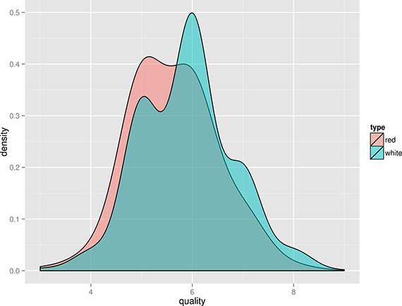
Figure 1. Comparing the quality of red and white wines using a density plot.
Does this mean that white wines are overall better than red wines, or that the white wine experts more easily give higher scores than red wine experts? That’s something that the data doesn’t tell us. Or is there perhaps a correlation between alcohol and quality? Let’s use Rio and ggplot again to find out (Figure 2):
$ < wine-both-clean.csv Rio -ge 'ggplot(df, aes(x=alcohol, y=quality, '\
> 'color=type)) + geom_point(position="jitter", alpha=0.2) + '\
> 'geom_smooth(method="lm")' | display
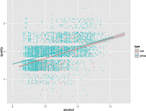
Figure 2. Correlation between the alcohol contents of wine and its quality.
Eureka! Ahem, let’s carry on with some dimensionality reduction, shall we?
Introducing Tapkee
Tapkee is a C++ template library for dimensionality reduction (Lisitsyn, Widmer, & Garcia, 2013). The library contains implementations of many dimensionality reduction algorithms, including:
- Locally Linear Embedding
- Isomap
- Multidimensional scaling
- PCA
- t-SNE
Tapkee’s website contains more information about these algorithms. Although Tapkee is mainly a library that can be included in other applications, it also offers a command-line tool. We’ll use this to perform dimensionality reduction on our wine data set.
Installing Tapkee
If you aren’t running the Data Science Toolbox, you’ll need to download and compile Tapkee yourself. First make sure that you have CMake installed. On Ubuntu, you simply run:
$ sudo apt-get install cmake
Consult Tapkee’s website for instructions for other operating systems. Then execute the following commands to download the source and compile it:
$ curl -sL https://github.com/lisitsyn/tapkee/archive/master.tar.gz > \
> tapkee-master.tar.gz
$ tar -xzf tapkee-master.tar.gz
$ cd tapkee-master
$ mkdir build && cd build
$ cmake ..
$ make
This creates a binary executable named tapkee.
Linear and nonlinear mappings
First, we’ll scale the features using standardization such that each feature is equally important. This generally leads to better results when applying machine-learning algorithms. To scale we use a combination of cols and Rio:
$ < wine-both.csv cols -C type Rio -f scale > wine-both-scaled.csv
Now we apply both dimensionality reduction techniques and visualize the mapping using Rio-scatter (Figure 3):
$ < wine-both-scaled.csv cols -C type,quality body tapkee --method pca |
> header -r x,y,type,quality | Rio-scatter x y type | display
Because tapkee only accepts numerical values, we use the command-line tool cols to not pass the columns type and quality and the tool body to not pass the header. This pipeline looks cryptic because these are in fact nested calls (i.e., tapkee is an argument of body and body is an argument of cols), but you’ll get used to it.
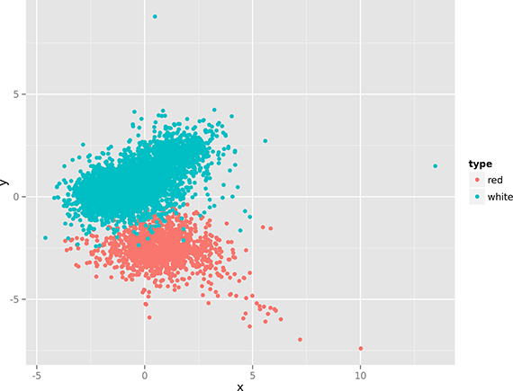
Figure 3. Linear dimensionality reduction with PCA.
$ < wine-both-scaled.csv cols -C type,quality body tapkee --method t-sne |
> header -r x,y,type,quality | Rio-scatter x y type | display
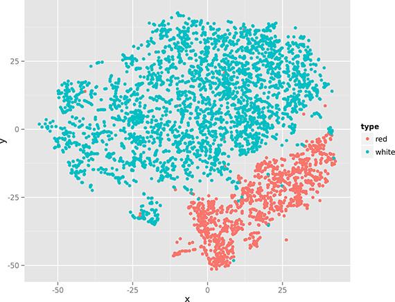
Figure 4. Nonlinear dimensionality reduction with t-SNE.
Note that there’s not a single classic command-line tool (i.e., from the GNU coreutils package) in these two one-liners. Now that’s the power of creating your own tools!
The two figures (especially Figure 4), show that there’s quite some structure in the data set, indicating that red and white wines can be distinguished using only their physicochemical properties. (In the remainder of Chapter 9, we apply clustering and classification algorithms to do this automatically.)
Conclusion
Dimensionality reduction can be quite effective when you’re exploring data. Even though we’ve only applied two dimensionality reduction techniques (we’ll leave it up to you to decide which one looks best), we hope we’ve demonstrated that doing this at the command line using Tapkee (which contains many more techniques) can be efficient. If you’d like to learn more, the book Data Science at the Command Line shows you how integrating the command line into your daily workflow can make you a more efficient and effective data scientist.